Applying an RMF

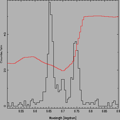
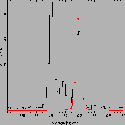
In the above example we were fitting a line where the ARF was constant across the region of interest. At the other extreme we need to fit lines where the arf is changing rapidly. In this case we need to use an ARF and RMF to convolve the model and fit to the data to get an accurate estimate of the line flux.

Figure 4: The Si line regin in the Capella spectrum with the arf (in arbitrary units) overplotted on the spectrum.

Figure 5: The Si line at 6.75 Åin the Capella spectrum with the fitted lsf shown in red.

For this example we need to load an ARF and assign it to a spectrum

isis>assign_arf(1,10);

Similarly, we need to load an rmf and assign it to a spectrum

isis> assign_rmf("acismeg1D1999-09-22rmfN0000.fits",10);

Get the ebounds array from the data

isis>(lo, hi, , ) = get_data(10);

Initialize the plasma database

isis> plasma ("aped");

Load a predefined model

isis> load_model("model.dat");

# id Temp Dens Abund Norm Vturb redshift Nh 
#     (K) (cm^-3) (km/s) (cm^-2) 
  1  2.0000e+06 1.0000e-03 1.0000e+00 1.0000e+00 2.0000e+02 0.0000e+00 1.0000e+20

and finally compute spectral model on the same grid as the data

isis> sp = model_spectrum (lo, hi);

Once we have loaded and assigned an ARF and RMF the fitting proceeds as above but this time the model is folded through the arf and rmf before being compared to the data.

To find the flux in the model,

isis> (lo, hi, dat, dat_err) = get_data(10); 
isis> (lo, hi, model) = get_model(10); 
isis> limits; 
isis> xrange(6.5,6.9); 
isis> hplot (lo, hi,model); 
isis>print,sum(model); 
0.00001527

MIT Accessibility