


Next: Determining a Line Flux
Up: Data Reduction
Previous: Examine the data
For this example we will work with the Fe line seen at 15A. First
lets enlarge the region near the line.
isis> xrange(14.99,15.07);
isis> plot_data(10);
and now we see the data as plotted in figure 2.
Figure 2:
The 15 ÅFe line in the Capella spectrum
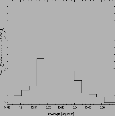 |
Figure 3:
The 15 ÅFe line in the Capella spectrum with
the fitted lsf shown in red.
 |
David Davis
2001-12-28
MIT Accessibility