| CSR Home Page: space.mit.edu/ |
MIT Chandra Science Center space.mit.edu/ASC/ |
Chandra Science: asc.harvard.edu/ |
Introduction
There are several targets in the in-flight calibration plan which are designated to check and verify effective areas (see HETGS simulations ). The brightest one of these is Cyg X-2. A 30 ks observation of Cyg X-2 may also allow us to check the HEG and MEG dispersion profile in the same detail as it was done during molecular contamination measurements at XRCF. The same observation will also be used to verify the effective area of the HETGS at energies above 1.5 keV. A short summary of the simulations presented here can be found at the official HETG simulations page. Please keep in mind that all the simulations are subject to change with every upgrade of the MARX simulator. While the official pages underly version control policies, this is an analysis site which will change on a continuous basis but which from time to time will also upgrade the official pages. Any portion on this page that is new with respect to the official HETG simulations page will be marked accordingly. . In any case this site will contain many more details which may or may not be interest to the observer.
The current set of simulations below were carried out with the MARX simulator version 2.15, which is still under development and not yet accessible to the public, but which offers several improved features such as an upgraded HRMA psf and a more realistic vignetting function. It however still utilizes a HRMA effective area model with 'old' optical constants which especially around the Ir-M-edges will significantly differ from reality.
Spectral characteristics of Cyg X-2
This bright LMXB is the prototype of the so-called Z-sources , which are persistently
bright X-ray sources that have distinct spectral states manifesting themselves in the
X-ray color-color diagram. For a more detailed reading we refer to the following
papers and references therein:
Schulz et al. 1989
Hasinger & van der Klis 1989
Wijnands et al. 1997
The input model for was provided by T. Kallman (GSFC) and is a result
of a detailed modelling of ASCA data based an the photoionization code
XSTAR. The model consists of three main components, two thermal
continuum components in form a 1.2 keV blackbody and a 5 keV cut-off
power law, and a third component describing an ionized photo-ionization
layer. A weak Fe-K line feature was also accepted in the ASCA fit.
A plot of the photon spectrums shown in
figure 1 , the data can be retrieved
in
table 1 . The source is fairly absorbed (NH=2.9x10e21 cm2) and will therefore
hardly contribute in the HETG below 0.8 keV. The spectrum below
that energy is too much affected by edges and lines and thus
the continuum structure is quite complicated. Some edges and line
are also expected to show up to 1.2 keV, above that energy, however, it
the spectrum is pretty much thermal continuum flux. The total flux
in the source spectrum amounts to 1.328 photons/cm2/s (or 5.6453E-09 ergs/cm2/s)
bwteen 0.11 and 10.0 keV. The flux below 0.8 keV is only
0.1422 photons/cm2/s1 (or 1.3827E-10 ergs/cm2/s).
The Simulation Set-up
For the simulation the MARX development version 2.15 has been utilized. For this version we pre-set the corresponding marx.par file in order to use custom defined detector quantum efficiencies and HETG efficiencies that have been recently tested during on ground calibration (see Absolute Effective Areas of the HETGS . The data file can be retrieved from the HETG home page . Every other parameter then should be set from the command line, for example:
"marx ExposureTime=30000 OutputDir='mydir' GratingType='HETG' DetectorType='ACIS-S', SpectrumType='FILE' SourceType='POINT' SourceFlux=-1 SpectrumFile='table1'"
One of the main intensions of this simulation is to characterize details expected from the instrument and separate them from expected discontinuous features in the source spectrum. We therefore constructed model spectra for each grating type and order, in which we folded the continuum components of the source spectrum with the instrument areas and efficiencies. Multiplied by exposure time and adjusted to the correct energy binning, the result serves as a perfect continuum model fit to the simulated spectra. Model spectra for HEG 1st and 2nd and MEG 1st and 3rd order are listed in table A . Note, that the ccd gaps appear in the model and in the simulated data, since for the time being, no dither motion has been applied.
Count Rates
Cyg X-2 is extremely bright and produces over 200 cts/s in 0th order and up to 3rd orders combined. Table 6 shows the expected count rates for the lower orders in MEG and HEG as well as the projected number of counts after 30 ks. A maximum flux of 0.04 cts/pixel/frame is reached around 1.6 keV in the MEG +1 and -1st order, which puts an upper limit pile-up occurrence to 1.5%. Table 7 shows a comprison of count rates in first orders of continuum and continuum plus line contributions. The expected line contribution to the total flux then is less than 2%.Dispersion Profiles and Residuals
Although we do intend to use the MEG 3rd and HEG 2nd order for higher order dispersion checks, for now we retrict the further analysis to the first order profiles only. Table B shows a set of profiles for the MEG and HEG first order in different energy ranges. The continuum fit is plotted as straight lines to highlist expected soucrce deviations, i.e lines and edges that are intrincic to Cyg X-2. All profiles are binned into single resolution cells of 0.048 mm bins, which offers maximum resolution of each grating.
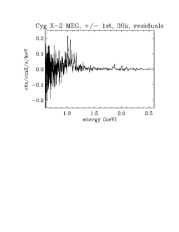
In addition
figure 18 shows residual spectrum of the MEG 1st order
at energies below 2.5 keV, which highlights
the sources deviations from the thermal continuum. Here we cleaned
the spectrum from grating effects. Therefore,
for example, no gap or Ir-edge mismatches are visible anymore.
This also allowed us to add positive and negative orders. The residual shows
quite a number of intrinsic lines around 1 keV and it is clear that in this
energy domain (< 1.2 keV) the
portion of the spectrum cannot be used for our purposes.
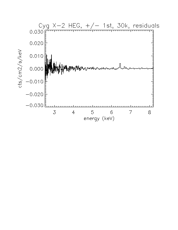
Above that energy, the residuals of the HEG 1st order (
figure 19 ) show a very clean spectrum, except for a weak F-K line at 6.4 keV.
Note, that the scale in figure 19 is already a factor 10 lower than in figure 18.
Spectral Variability
|
Norbert's In-Flight home Accessibility |