Revision status
Last revision in version control:
- Author: hamogu moritz.guenther@gmx.de
- commit 8d4d4d9c1ede3848f458ca3d1dd1380a03c7df86
- Date: Mon Oct 4 11:50:24 2021 -0400
This document is git version controlled. The repository is available at https://github.com/Chandra-MARX/grating-insertion. See git commit log for full revision history.
Code was last run with:
MARXS ray-trace code version 1.3.dev44 (commit hash: 05872a3) (Date of dirty version: 20210913)
Ray-tracing incomplete Chandra grating insertion
I present ray-traces of Chandra gratings that are not fully inserted. The simulations concentrate on the effect of the insertion angle and do not treat other effects that also reduce the resolving power in Chandra grating spectroscopy (such as uncertainties in aspect blur or the finite spatial resolution of the detectors). Taking this into account, a grating insertion error of order 0.5 degrees will noticably broaden the LSF; larger dispersion angles (longer wavelength and higher orders) suffer more from the error. This work was motivated by a grating insertion failure in summer 2021, to develop contingencies in case a modified grating insertion procedure may not produce fully repeatable positions. However, the insertion failure turned out to be caused by a temperature effect in the electronics which can be accounted for, such that the gratings DO insert to the correct position. Thus, fortunately, the work below remains a theoretical study with no direct application to Chandra data and I have left a few questions open that would require significantly more work to answer.
All the 3D views below are interactive if you view this on a website. They can be rotated, panned, and zoomed with the different mouse in all supported browsers; for trackpad users hold down CTRL or ALT for pan and zoom. Pressing "r" on the keyboard when the mouse is on a view returns that particular view to the initial position. See the X3DOM documentation for a full list of supported mouse and keyboard commands.
Notebook initialized with x3d backend.
Simulation setup
We usually use the marx code to ray-trace gratinga on Chandra. Unfortunately, the internal structure of the code requires significant changes to rotate the grating support structure in the way we are discussing here. Thus, the simulations shown below use the marx mirror model, but simulate gratings and detectors with the MARXS code, a Python ray-trace code I have written for the simulation of Arcus, Lynx, and a other missions. MARXS is explicitly designed to study misalignments of parts and, in fact, I have used it before to study the requirements on the repeatability of the grating insertion for Lynx in a setup very similar to what I present here.
That said, MARXS does not have the same fidelity for Chandra that marx has. In particular, it does not treat the characteristics of the detectors such as ACIS event grades or the HRC contributions to the point-speard functions. While it could simulate the Lissajous pattern of the Chandra pointing, MARXS does not (yet) write all the required keywords to run the event files it produces through CIAO for aspect reconstruction. So, at this point, the simulations below do not include all effects that influence the resolving power of the gratings in a real Chandra observation. However, they do describe how the LSF changes when the gratings are not fully inserted, which is what we want to study here. That is not an unreasonable approach: By ignoring the additional blurring of the LSF that stems from uncertainties in the aspect solution, the finite time resolution of the asol files and the ACIS readout (which contributed about 0.1" blurring for the standard 3.2 s ACIS read-out time), and the detector characteristics (event grade, HRC non-linearities in scale), we can isolate the effects that stem from changes in the grating position.
To further simplify the analysis, the simulations use an ideal, curved detector that follows the Rowland circle exactly, while HRC-S and ACIS-S are made up of several flat parts. This way, we do not have to worry aobut one of the simulated wavelengths hitting a chip gap. In that sense, all the numbers presented below for resolving power, effective area etc. are upper limits.
At this time, I am still missing some crucial input data for the LETG: I do not have a table of the exact locations of the facets. Therefore, the LETG simulations are performed by assuming the HEG and MEG facet locations, but with the LEG period and rotation angle. This impact the total effective area, but not the relative change of effective area with the grating insertion angle and will have a negligible effect on the resolving power, which is the main concern here.
Also, the location of the grating hinges is not fully correct, it's estimated from an unscaled drawing. I expect this to be good to about 5 mm; good enough that it will not change the results presented here.
HETG
First, I am looking at the HETG. The reason for that is simply that the HETG is more fleshed out in MARXS. I do not expect any of the main conclusions to change from the additional simplifications made for the LETG simulations below, but it still seems sensible to do the most detailed analysis on the instrument where I have the most detailed input information.
Geometry
Monoenergetic (1 keV) simulation of the HETG in nominal position. Active grating area is shown in white. Additionally, the HETG is shown rotated by 10 deg. In practice, the positioning will be much better than that, but this large rotation makes it easy to see in which directions the gratings are displaced to check the setup of the geometry. The curved yellow surface marks the location of a large, ideal detector following the Rowland circle. Zooming in on the focal plane, the 6 chips of ACIS-S are also visible.
Line profiles
I first show how the line profiles change for a few examples. This is a simulation with 1 keV photons. The plots below show the photon distribution in order -1 for the MEG and HEG. Note that the x and y axes are scaled differently. At this energy, the HEG data is not typically captured in a standard setup, but it can serve as an example of line shapes at larger distances from the focal point.
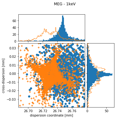
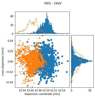
In both plots, the blue points and histograms are for the nominal position of the HETG, the orange symbols and histograms are for a grating insertion error of 0.5 deg. Shapes in the HEG and MEG are similar, but more extreme in the HEG because of the larger dispersion angle. If the grating is not fully inserted, the center of the distribution is at smaller dispersion coordinates and the shape approaches the outside of a square. This shape can be understood as follows: The Rowland torus is designed in such a way that rays have the best possible focus in dispersion direction at the detectors. Even for a misaligned grating, that is still true for some gratings since the gratings located closest to the yoke move only very little. On the other hand, the gratings furthest from the yoke move significantly more and thus photons coming from those gratings will be significnalty out of focus. Because the yoke is angled with respect to the dispersion direction, the resulting shape is not symetric to the dispersion either.
In the following sections, I simply use the standard deviation $\sigma$ as a measure of how wide each line is and estimate the resolving power as $R = \sigma/\Delta x$, where $\Delta x$ is the distance between the zero order and the mean location of the photons of this wavelength. A very detailed analysis using the predicted more complex line profiles as LSF when fitting spectra might be able to recover more information, but for the present purposes, it is sufficient to simply take the standard deviation as a measure of the width of the LSF.
Working on simulation 0/11
/Users/hamogu/code/marxs/marxs/optics/grating.py:248: RuntimeWarning: invalid value encountered in arccos
  n)))
Working on simulation 1/11
Working on simulation 2/11
Working on simulation 3/11
Working on simulation 4/11
Working on simulation 5/11
Working on simulation 6/11
Working on simulation 7/11
Working on simulation 8/11
Working on simulation 9/11
Working on simulation 10/11
Working on simulation 0/11
Working on simulation 1/11
Working on simulation 2/11
Working on simulation 3/11
Working on simulation 4/11
Working on simulation 5/11
Working on simulation 6/11
Working on simulation 7/11
Working on simulation 8/11
Working on simulation 9/11
Working on simulation 10/11
Working on simulation 0/11
Working on simulation 1/11
Working on simulation 2/11
Working on simulation 3/11
Working on simulation 4/11
Working on simulation 5/11
Working on simulation 6/11
Working on simulation 7/11
Working on simulation 8/11
Working on simulation 9/11
Working on simulation 10/11
Resolving power

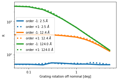
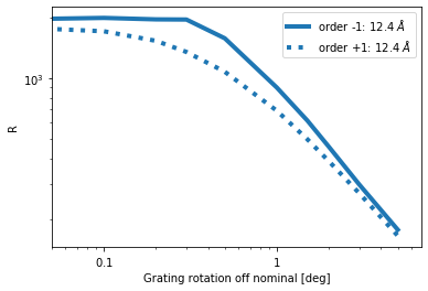
Resolving power for HEG (solid lines) and MEG (dotted) with insertion angle error. In the nominal position (angle=0 deg), the resolving power for a given order depends linearly on the wavelength, simply because photons of longer wavelength are diffracted to larger angles. The same holds to photons of different orders: $R$ increases with order.
Note that in practice Chandra does not reach the highest resolving powers shown in the figure above for several reasons. Long wavelengths and higher orders may not actually fall on the ACIS array. For example, the highest $R$ values shown are for third order photons with $\lambda > 12$ Ang, which do not fall on the ACIS chips. Similarly, the efficiency for longer wavelength in the HEG is so low that no usuable signal is collected in practice.
Furthermore, the simulations here ignore a number of other effects that reduce the resolving power, e.g. uncertainties in the aspect solution, the difference between flat gratings and the ideal curved Rowland circle, or the finite pixel size of the detectors. The goal here is to see when the rotation of the HESS becomes the dominant effect on $R$. While I do not include all those other effect in the simulations here, we can assume that they roughly add up in quadrature; whatever the details of this, the final $R$ will always be lower than the number shown here due to these effects. Because of this, the values for R shown in the figure above are higher than what the real Chandra provides.
The resolving power starts dropping noticably aroud 0.3 deg and falls dramatically above 1 deg or so. Longer wavelength and higher orders start to suffer earlier. It is interesting to see that for larger errors in angle $R$ does no longer depend on wavelength or diffraction order because the line broadening introduced by the error in grating position grows with the diffraction angle.
In the plot above, positive and negative orders are averaged. However, for a rotated HESS, positive and negative orders are no longer symmetric. One set of spectra is now under the "high" side of the HESS and the other one is located under the "low" side. This causes small differences in the line profile, which can be seen in the simulations.
For no rotation, the resolving power $R$ is (up to the noise in the Monte-Carlo simulation) identical in the positive and negative orders of the MEG. With increasing rotation, one side performs better than the other one, until the roation becomes very large.
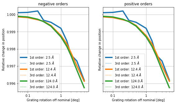
Wavelength solution
When the HESS is the not in the correct position, the gratings will be on average futher from the mirror and closer to the focal plane. That means that the light rays go through the mirrors later and, even if diffracted by the same angle, don't make it as far away from the zero order. One can think of this as a smaller average Rowland circle. This effect can be calculated analytically, but the simulations show it, too.
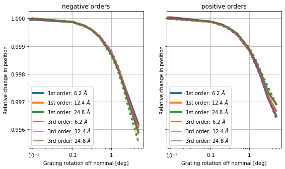
There are slight differences between the positive and negative orders, because the geometry is not symmetric when tilted, as the HESS now has a high side and a low side. In both cases, the differences are of order 0.1% at 1 deg or about 300 km/s.
So, unless the insertion error is significantly below one degree, this is in the range we need to worry about, in particular, because this is systematic. Since the gratings will never be rotated too far, but always too low, every Chandra observation would indicate smaller diffraction angles (i.e. shorter wavelength).
In some observations, the wavelength solutions can be obtained from the observation itself (self-calibration). Today, this is only done for calibration observations (Capella), but in principle this can be done for any observation with features at a known position, or for any observation where the same feature is observed in both first and third order (I'm not writing down the full math here, but seeing the same feature in two orders gives us an extra piece of information, which we can use to solve for the angle of rotation of the HESS). However, in the vast majority of observations, we will need to rely on a known wavelength solution.
Loss of photons / Changes in effective area
Currently the code does not have information how the grating efficiency changes with infall angle. The HETG ground calibration report (figures 4.11 and 4.12) indicates that these changes are large, but linear at about 7%/deg for the MEG and 35%/deg for the HEG. We expect this effect to almost exactly cancel out due to the way the HESS is populated with gratings. Gratings are manufactured for a specific sector and are thus marked as A, B, ..., but there is no difference in the grating mounts between gratings mounted in sectors A and AA, or B and BB etc. Since gratings in opposing sectors A and AA are rotatated by 180 deg with respect to each other, we expect that any loss in effective area in sector A is exactly compensated by a gain in AA for any particular order.
What is easy to check in ray-tracing is if a photons actually hits a grating membrane or if it hits a frame instead. I call this the geometric area of the gratings and this is shown in the next plot.
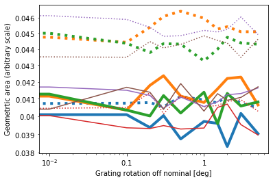
Shown is the geometric area of the grating. Note that the y axis has an arbitrary scale, only the change of area with angle is significant. (I could normalize all curves to 1 at angle=0 deg, but then they would be hard to see because they are all plotted on top of each other.) Colors and line styles are identical to the figure "R vs. angle" above.
The change in geometric area shown here differs from the effective area as is does not take into account any change in diffraction efficiency for photons that do not arrive perpendicular to the grating surface. Instead, this is a simple geometric area (on an arbitrary scale). This area is constant within the noise of the Monte-Carlo simulation. That means that we are not yet loosing photons because they hit the frames instead of the active surface. For angles as small as we discuss here that is the expected result since the gratings only move by a few mm; much less that their physical size. Still, it is good as a cross-check for the validity fo the simulation.
LETG
Results for the LETG should be very similar to the HETG results, except that the LETG usually uses the HRC-S which reaches to larger diffraction angles. Thus, I show only a subset of the figures I presented for the HETG. Nevertheless, I think that the simulations I present here are sufficient to answer the core question "How much tolorance on the exact insertion angle can we tolerate?"
See the section on the HETG above for a detailed description of the figures.
Working on simulation 0/11
Working on simulation 1/11
Working on simulation 2/11
Working on simulation 3/11
Working on simulation 4/11
Working on simulation 5/11
Working on simulation 6/11
Working on simulation 7/11
Working on simulation 8/11
Working on simulation 9/11
Working on simulation 10/11
Working on simulation 0/11
Working on simulation 1/11
Working on simulation 2/11
Working on simulation 3/11
Working on simulation 4/11
Working on simulation 5/11
Working on simulation 6/11
Working on simulation 7/11
Working on simulation 8/11
Working on simulation 9/11
Working on simulation 10/11
Working on simulation 0/11
Working on simulation 1/11
Working on simulation 2/11
Working on simulation 3/11
Working on simulation 4/11
Working on simulation 5/11
Working on simulation 6/11
Working on simulation 7/11
Working on simulation 8/11
Working on simulation 9/11
Working on simulation 10/11
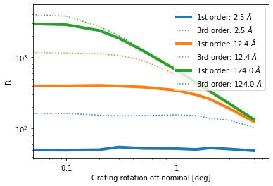
Similar to the HETG, the LETG resolving power increases with wavelength and this order. Like the HETG, the LETG does not reach the theoratical maximum because of other limitations (uncertainty in aspect solution etc.). Taking this into account, an insertion error below 0.5 deg or so is probably tolerable for the LSF, above that value $R$ will decrease for long wavelength.