Fitted LSF Parameters

The simulated line profiles, from MARX, are fit with a Gaussian plus Lorentzian profile.

(1)

where r₀ is the peak of the Gaussian, is the Gaussian width and r is the distance from the peak. For the Lorentzian component is the Lorentzian width, r is the Lorentzian center not necessarily the same as the Gaussian peak, and a-0 is the relative normalization with respect to the Gaussian. 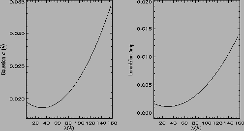Figure 6 shows the variation of the Gaussian and relative Lorentzian normalization as a function of wavelength while figures 7 and 8 shows the same for the HEG and LEG spectra.

 

Figure 6: MEG Gaussian Width and Lorentzian amplitude vs wavelength

 

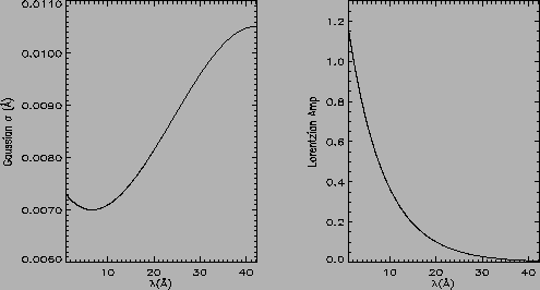Figure 7: HEG Gaussian Width and Lorentzian amplitude vs wavelength

 

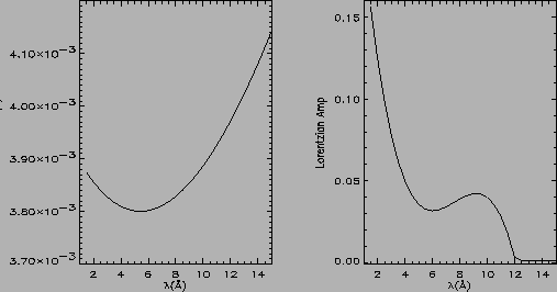Figure 8: LEG Gaussian Width and Lorentzian amplitude vs wavelength

In these fits the Gaussian peak is set to 1.0 and the Lorentzian is fixed at 0.012 Å.

As can be seen in figure 6 the Gaussian width between about 10 and 40 Årises from a low of 0.007 to a high of about 0.0105 Å. The right panel shows the Lorenzian amplitude (relative to the Gaussian) as a function of wavelength. At long wavelengths the Lorentzian is a weak component but at short wavelengths the Lorentzian component dominates over the Gaussian component. This effect is expected and is mostly due to mirror scattering (see POG figure 4.6) and so the scattered component, represented by the Lorentzian, dominates at short wavelength (high energy).

MIT Accessibility